Introduction

Electrical power lines carry an electrical current, whereas a magnetic field is produced from the conducting wire which induces an AC voltage into the buried pipe. This linking causes an alternating voltage and current to be induced onto a parallel collocated pipeline.

When a pipeline located near a power line, it is subject to several electrical effects depending upon the operational status of the line. In addition, a lightning stroke or other cause, the power line will experience a short circuit condition known as a fault. The focus of the AC predictive guide is based on inductive/conductive coupling and fault conditions from co-located power lines using ACPT.

AC Pipeline Prediction Fundamentals

Understanding AC circuits and prediction fundamentals is a must. (See TT’s Website on Training for AC Mitigation). The ACPT focuses primarily on inductive and conductive (resistance) and not on capacitive interference effects.

Electrostatic Interference:

• Capacitive when pipe is above ground
• Function of voltage not current
• Transfer of small amounts of power to pipeline
• Can result in high voltages on short sections
• Considered nuisance voltages

Electromagnetic Induced Voltages:

• Function of tower current, not voltage
• Power transfer is proportional
• Line current
• Longitudinal Electric Field (LEF)
• Length of parallelism
• Inverse to the separation distance
• Results in high voltages on long sections of pipeline

AC Faults – Inductive & Conductive

• Rare in the US
• Short duration (micro to milliseconds)
• Weather conditions
  • High winds
  • Lightning
• Structural failure
  • Poor maintenance
  • Accidental damage
  • Vandalism/Terrorism

AC Mitigation Understanding

AC mitigation is a way to reduce the effects of induction from the effects of AC power line interference. This is accomplished by using ground principles. See section 5 for more information.

Types of Mitigation or Grounding

• Discrete Anode
• Distributed Anode
• Linear wire or cable (Copper or Zinc)

  AC Decoupling Devices, Polarization Cells, and Surge Protection

• Dairyland Devices (See Appendix B)
• Copper Cable for Parallel Grounding
• Distributed Ground Beds
• Discrete Ground Beds

  Mitigation to Meet NACE Standards

• Less than 15VAC (Personnel Safety)
• Personnel Hazard

Gradient Control Mats at Pipeline (Personnel Safety)

• Appurtenances such as Test Stations & Valves
• Grid mats with Zn, Cu
• De-couplers

Practical Approach to Mitigating Corrosion

Induced AC Potentials

• Induced AC into a pipeline or to earth is directly proportional to the strength of AC tower current load
• Inverse distance between parallel structures
• Pipe diameter
• Coating conductance/resistance
• AC tower loads (Seasonal)
• Longitudinal electrical fields (LEF) are induced into the earth
• LEF can be field measured to estimate AC before a pipeline is constructed

Discontinuities – Physical Pipeline

• Approaches or recedes from power line R/W
• Changes distance from power line circuit
• Crosses under power lines
• Contains an isolating device
• Transition from below to above ground
• Significant coating resistance change

Discontinuities – Electrical Tower Line

• Power line transpositions
• Change in powerline configuration
• Addition or removal of power line
• Changes in LEF (pipeline) at a faulted tower

Tower Data

Additional data are required for the average tower ground resistance to remote earth and the average separation between the faulted transmission line towers (structures).

Cross-sectional height and horizontal displacement of the shield (sky) wires from the tower center line are evident inputs. Program default accepts data for two wires with the assumption that the wires are periodically grounded to the tower grounds. However, this is not always the case.

Physical placement of the wires, i.e., height and horizontal displacement from the tower center line are obvious when data are available. Default values for typical circuits as a function of circuit voltage level are available from within the program database.

Below are typical fault current values, separation tower distances for the circuit voltage in kV. There are four (4) primary power transmission line types: (See Appendix C for Field Data Requirements)

• Single Horizontal
• Double Horizontal
• Single Vertical
• Double Vertical

The tower voltages run from 69 kV to 550 kV. For example, if the tower voltages are lower than 69 kV, the 69 kV-100 can be used; however, the correct current load must be obtained from the power company.

Power transmission operating data are not always available from Power Companies. Although the program gives operating defaults, these values must be verified especially with day-to-day loads which directly impact the induced steady-state voltages on the pipeline. Below is a table that shows the ranking of the current loads on a pipeline right of way in Table 1.

Table 1 – Relative Severity of AC Interference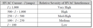

Fault conditions from co-located power lines also present inductive/conductive conditions on the pipeline. Below is table 2 that provides typical tower voltages, currents, and separation that are required for input to the ACPT program. These data should also need to be verified by the Power Company.

Table 2 – Tower Circuit Fault Voltages and Currents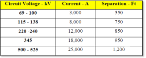

Bulk Soil Layering (Barnes Layer)

Barnes layer data are set up to represent the bulk soil multiple layers for the corrosive layer (pipe depth), apparent layer (steady-state and inductive fault), and conductive layer (conductive fault). Other considerations include:

• Where soil resistivities are not deep and change i.e. from deep tower footing grounds compared to the shallower pipeline trench, faults may stress the coating.
• Where these conditions exist, running multiple scenarios at the fault tower(s) is needed to assess for various depths.
• For example, using the Barnes Layer in areas where there are deep HDD crossings is recommended. Adjustment to the spreadsheet calculations may be needed to accommodate these depths for a more accurate assessment of these layers.
• In HDD crossings, it should be noted that drilling muds contain bentonite clays that have very low resistivities in the range of 100 ohm-cm. The soil resistivity meters may, or in most cases may not detect this narrow layer of the drilling muds around the pipe.
  • If the backfill is typical soils, the drilling muds will migrate into the soil after several years.
  • If the backfill is in granite or similar rock, the muds may remain in place for many years.

Note: Barnes Layer – Below is a typical schematic of these three (3) major layers to consider bulk and specific layer resistivity. Any of these layers can be varied in depth depending on the geo layering and resistivity layers related to pipeline depth.

See attached as an example Excel Spreadsheet to set up multiple layers at the end of this manual.

Note: There are soil resistivity inversion programs that calculate a two-layer method based on field measurements and depths. Technical Toolboxes allows the user to select the methods of measurement and calculation methods for data input.

Example of Barnes Multi-Layer Soil Resistivity for AC Modeling and Mitigation: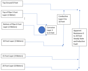

Pipeline Data Required (Manual Entry)

Diameter

Coating Resistance (See Coating Resistance Tables in Section 2.9)

Depth of Cover per section

Soil Resistivities (See Barnes Layer Spreadsheet)

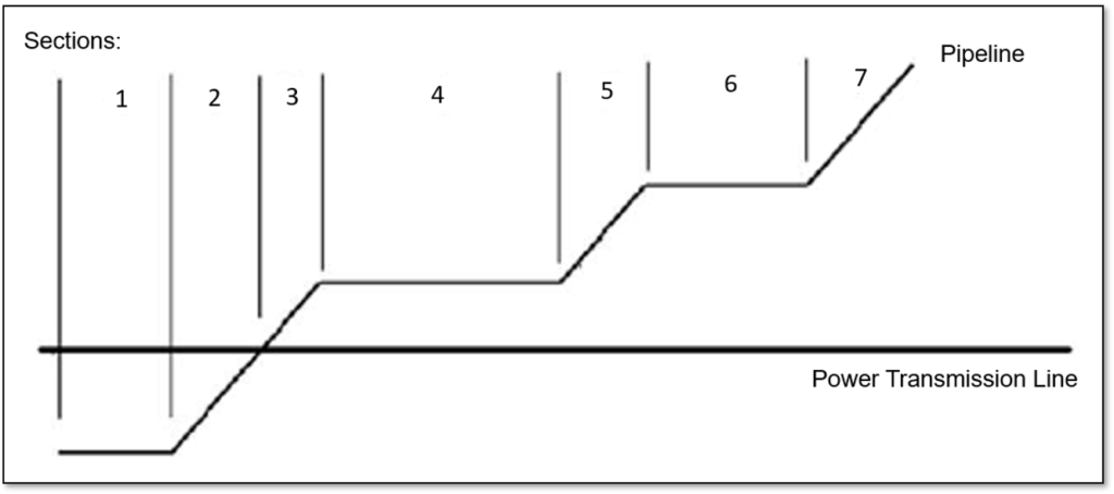
Pipe Sections (Manual) are shown below. (See section 7 (Users Guide) for additional information in setting up and adding sections).

Angles should be similar to pipeline angles i.e. section 1 (45 degrees ahead and to the left towards the power line. Section 3 (45 degrees ahead to the right).

Distances from pipe to tower should be based on which side of the pipe is relative to the power line i.e. (Section 1 is 50 feet from pipe to power line). Since there is a tower at section 2, it is the distance from pipe to tower i.e. 10 feet. Section 3 example is set -25 feet from pipe to tower.

The same concept applies to the remaining line sections 4, 45 degrees ahead to the left at -25 feet and section 5, 45 degrees right at -75 feet, etc.

Pipeline Sections Creation

Four (4) Types of Importing LAT./LONGS and GIS Data

• Shape Files (shp.)
• Map File (kmz. & kml.)
• Create from GIS
• Excel

For example, A map kmz. or kml. file was imported for both the Power Transmission Line and Pipeline as shown on the next page. Then point and click technology is used to create sections at nodes, towers, proposed mitigation sites, soil resistivity changes, transpositions, etc., Once this is completed, the user can calculate sections, distance, and angles.

The ACPT automatically calculates:

• Proximities to each structure
• Angles to each structure
• Section lengths based on engineering criteria
• Depth of cover (DOC) imported to each section as needed

This workflow allows the user to import large data sets quickly for pipelines and AC transmission lines. By using Point and Click which sets up sections within minutes and identifies AC threats immediately start design mitigation strategies. If you need to put in an additional section or sections, just go back and insert with no limitations.

Related Links

AC Mitigation PowerTool