Example: Importing DXF & Working with Shapefiles

Contents

These worked examples build a complete model from a DXF file, check and correct its connectivity, project a model between longitude/latitude and plane coordinates, and cover the background on working with shapefiles (SHP). Set your default data values before importing — anything not captured by the source file falls back to those defaults, and correcting them afterward across many features takes far more effort than setting them up front.

Import A DXF File (Example)

Creates a model from a DXF file by importing its pipe line work, using the same file as the model’s background image, then checks connectivity with Trace, solves, and reviews the results.

1) Set The Default Data Values

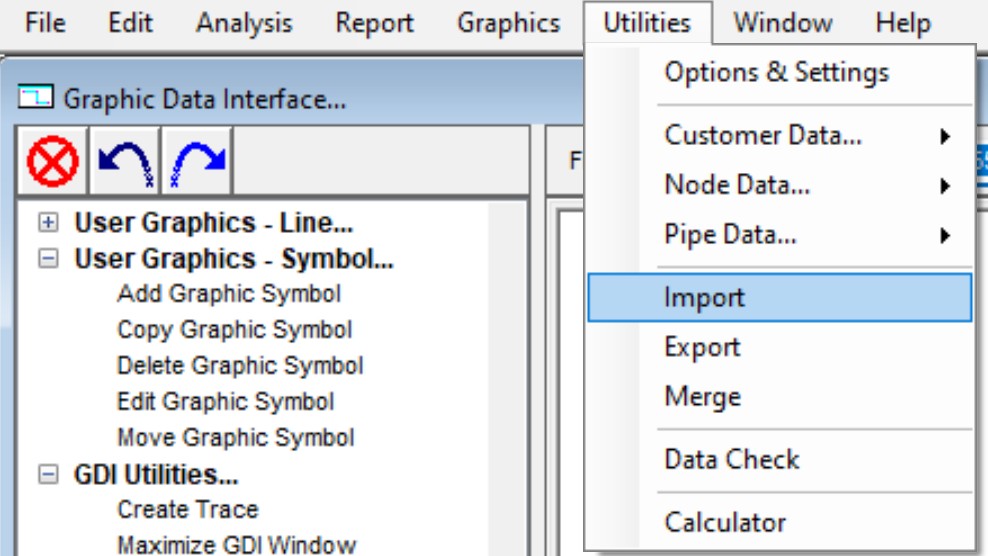
From the Utilities menu, select Import. On the Save screen, type a new model File name and click Save. On the Import screen, click Set Default Data Values.
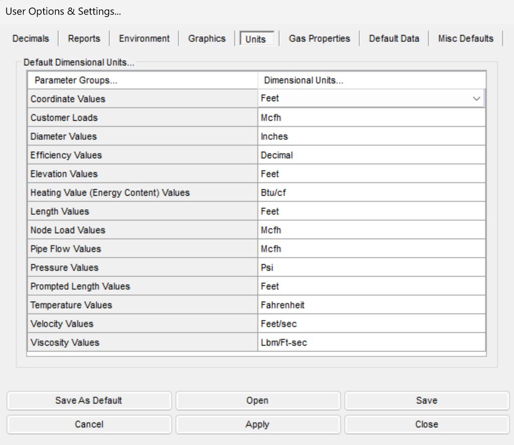
On the Units data tab, set the dimensional units for the model — for example, Coordinate Values to Feet, Diameter Values to Inches, Pressure Values to Psi, and similar choices for the remaining Customer Loads, Efficiency, Elevation, Heating Value, Length, Node Load, Pipe Flow, Prompted Length, Temperature, Velocity, and Viscosity items.
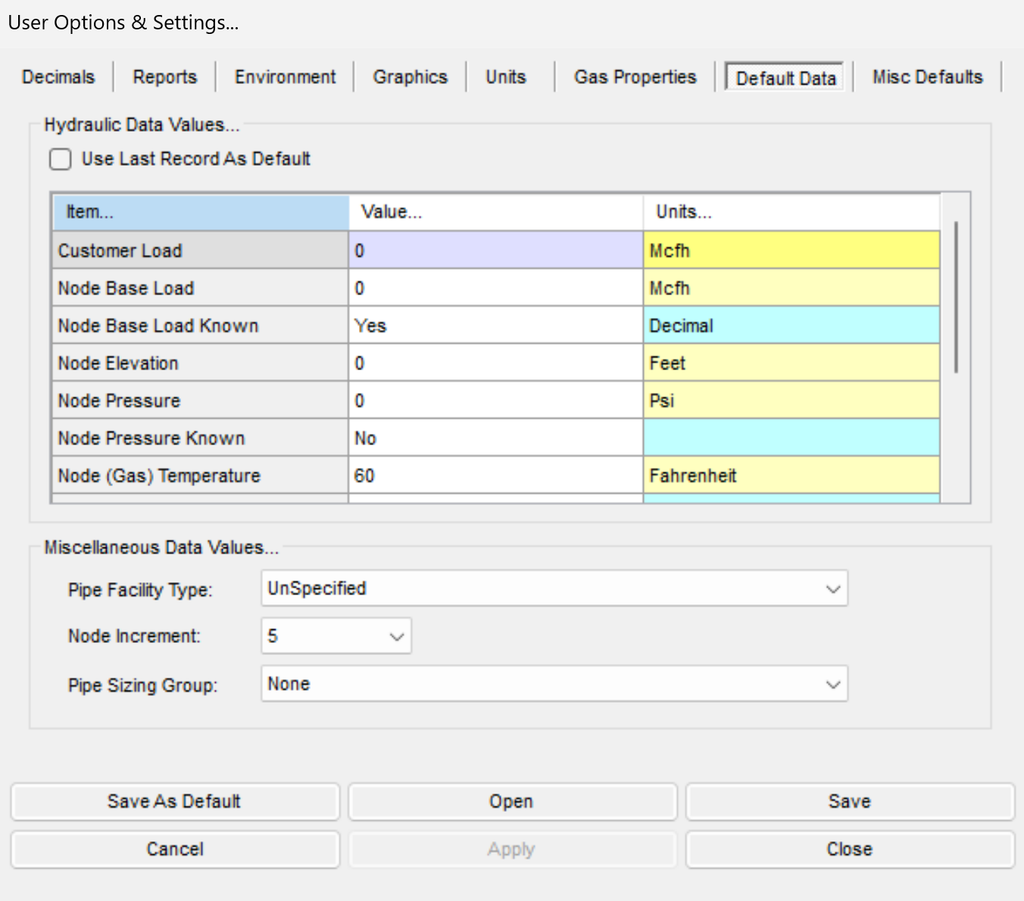
On the Default Data tab, set starting values for new features — for example, a small negative Node Base Load to get started, Node Pressure Known set to Yes, Pipe Flow Equation set to IGT-Improved, Pipe Hydraulic Efficiency set to 0.95, and an out-of-range Pipe Size/Type value (such as 99 inches) to help flag pipes that don’t get a diameter assigned automatically during import.
On the Gas Properties data tab, set the Default Gas Property Values — Specific Gravity, Viscosity, Heating Value, and Specific Heat Ratio — for the gas being modeled.
Click Close to return to the Import screen.

2) Import The DXF File

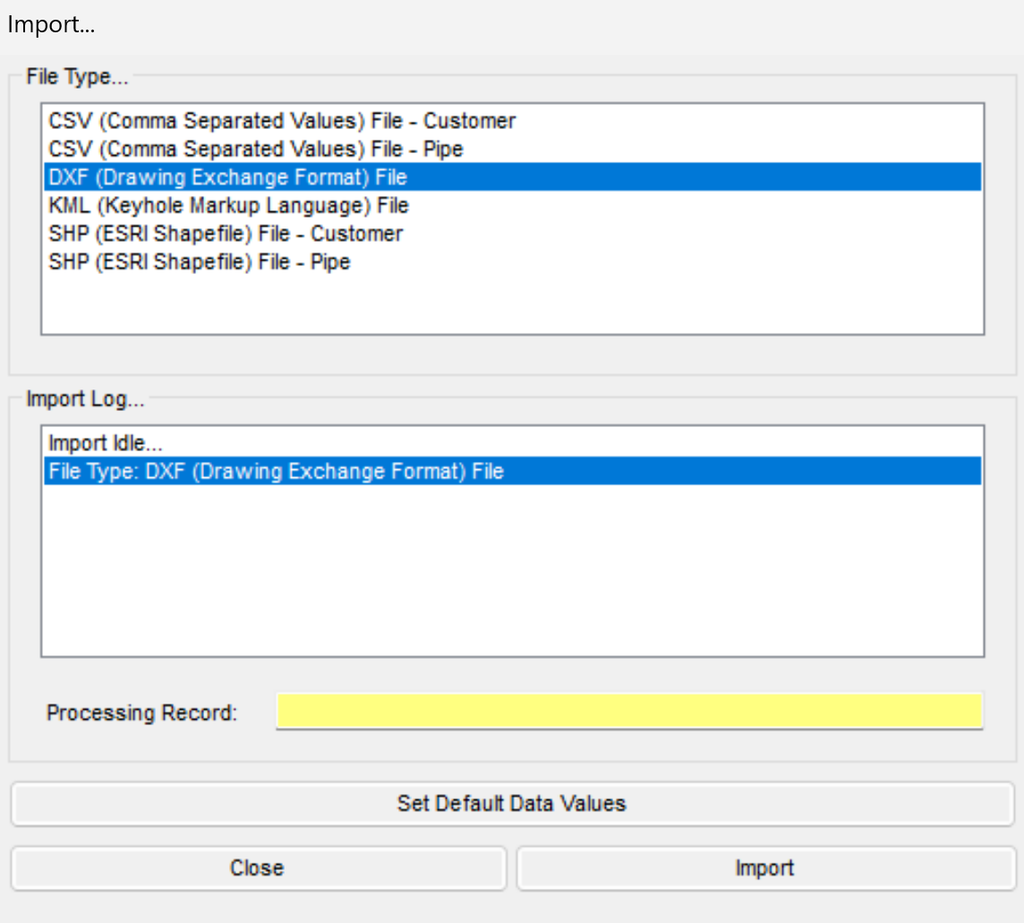
On the Import screen, select “DXF (Drawing Exchange Format) File” from the File Type list and click Import. Select the source .dxf file and click Open.
On the Import Specifications screen’s Pipe Settings tab, assign each DXF pipe layer to its corresponding Pipe Size/Type, set the Fuzzy Tolerance and Pipe Length Units, and set the Drawing Coordinate Units and any Origin Shift needed.
Click Continue. When the Import Log reports completion, click Close to return to the GDI Window.
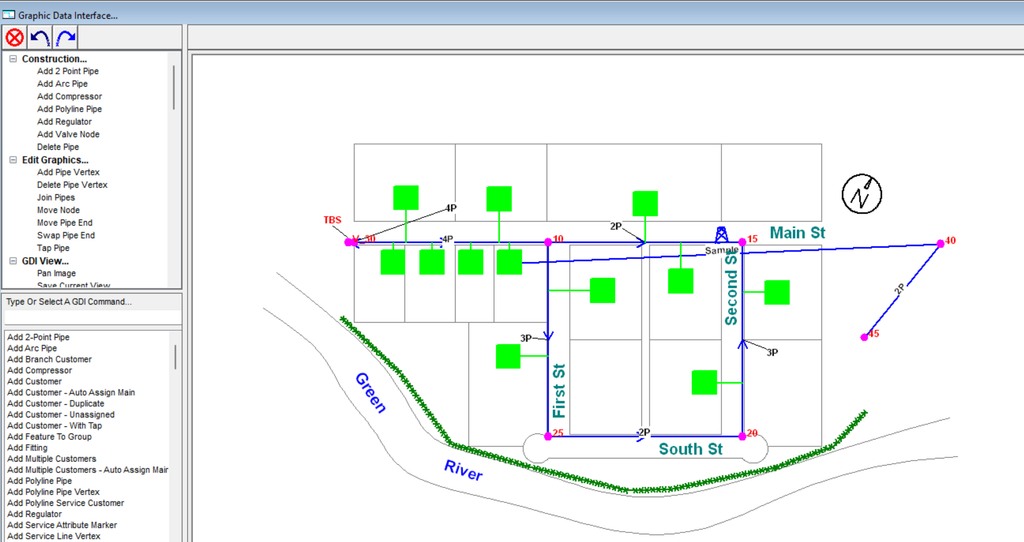
Maximize the GDI Window (GDI Utilities branch of the GDI Command Tree) and click Zoom To Fit.

3) Set The Graphic Settings

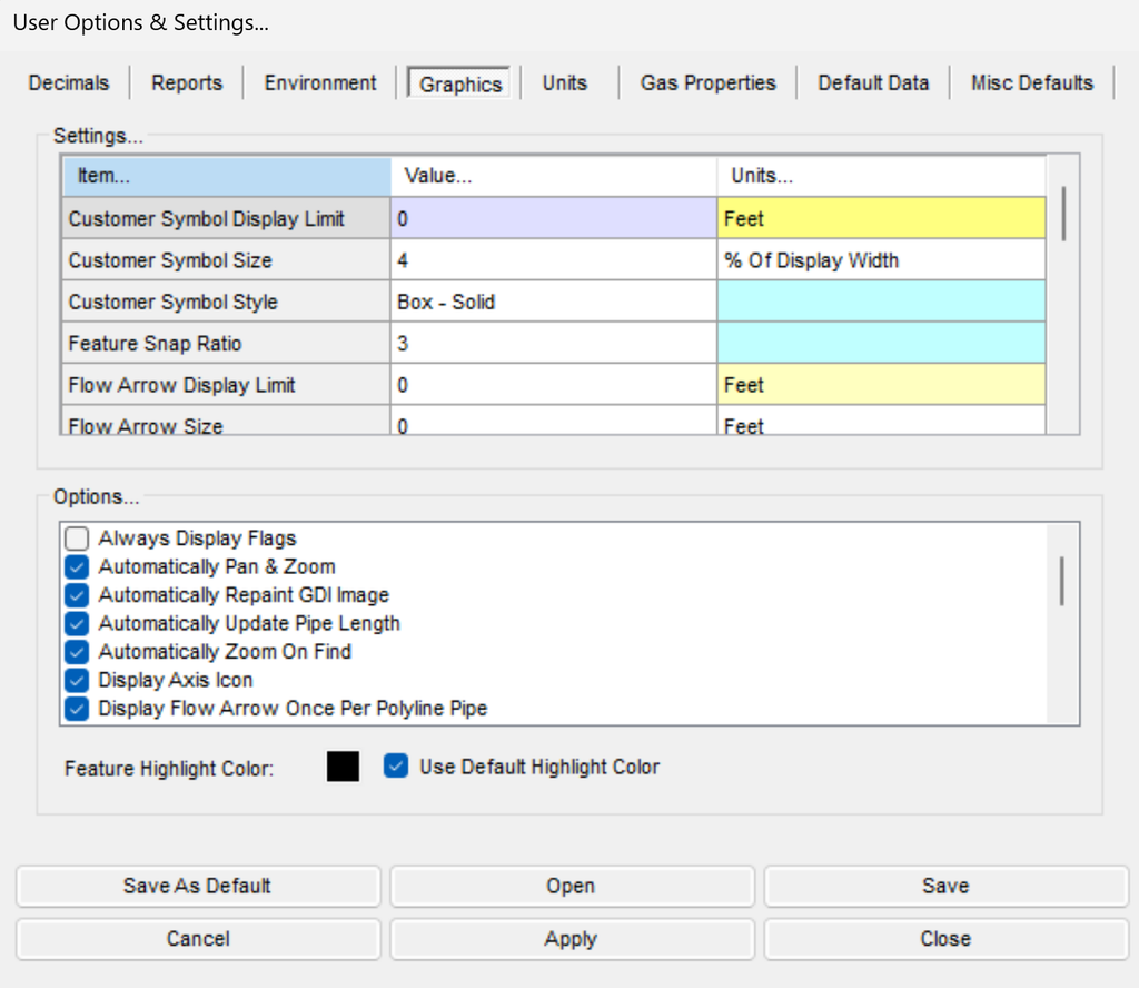
From the Utilities menu, select Options & Settings.
On the Graphics data tab, set Node Symbol Size to a percentage of display width (1% works well for most models).
On the Environment data tab, select Prompt For Data During New Feature Entry.
Click Apply, then Close.

4) Attach The Background Image

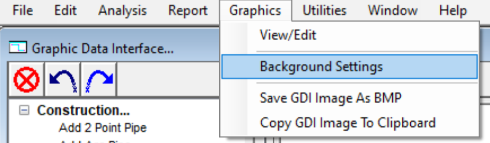
From the Graphics menu, select Background Settings, then click Attach New Image.
On the Attachment File Type screen, select “DXF – Drawing Exchange Format Style CAD File” and click Continue.
Select the same .dxf file used to import the model and click Open.
Click Apply on the Background Image Settings screen. If the image doesn’t appear, select Display Background Image from the Display Settings branch of the GDI Command Tree.

5) Check & Edit The Model Connectivity

Select Create Trace from the GDI Utilities branch of the GDI Command Tree. Set Trace Style to “Trace All Directions,” Start Trace At to “A Node,” and pick a Trace Highlight Color, then click Trace.
At the Select Starting Node prompt, click the node at the supply end of the system. If the trace stops partway through the model, zoom into the point where the color changes to investigate.
If a piece of equipment is missing at that point — for example, a regulator between a supply line and the distribution system — add it: select Add Regulator, set its From and To nodes, size, control style, and set pressure, then accept the new pipe data.
Set the outlet node’s Pressure Known value to “Yes” in the Data Panel, and click Apply Data Values.

6) Recheck The Connectivity

Click Zoom To Fit, then run Quick Trace from the GDI Command List to recheck connectivity.
If a lateral pipe still isn’t colored, zoom into its end to check whether it’s actually connected to the header pipe it appears to touch.
If it isn’t, use Tap A Pipe (Edit Graphics branch of the GDI Command Tree): select the header pipe, then click the location of the disconnected end to split the header and join it there.
Retrace from that point and confirm the entire system now colors correctly with a final Zoom To Fit.

7) Set The Non-Default Pipe Data

Left-click the supply line and, in the Data Panel’s Hydraulic Data Items, set its correct Hydraulic Length and Length Units, then click Apply Data Values.
Left-click the node at the supply end of the line and set its Pressure, Pressure Units, and Pressure Known values in the Data Panel, then click Apply Data Values. The example ends here — later steps like adding customers and solving the model are covered in their own topics.

Notes

This example used a well-prepared DXF file — pipes snapped together, broken at intersections, and grouped onto correct layers. Real drawings aren’t always this clean; while GASWorkS can edit piping data after import, it’s better to fix problems in the original DXF file so a future re-import doesn’t require redoing the same corrections.
This drawing was already to scale. GASWorkS can scale and rotate a model after import, but scaling the original DXF file first is preferable — and if the model is scaled after import, the background image must be scaled to match, or it won’t display correctly.
Good DXF preparation habits: draw to scale; use decimal or engineering notation rather than architectural notation; snap pipe ends together; break pipes at connected intersections; group piping by size and material on separate layers; keep only pipe lines (no symbols or blocks) on the pipe layer; and put valve nodes on their own layer with a consistent block symbol.
This example only did a cursory connectivity and pipe-size check. Before relying on an imported model, check every pipe size and connection carefully — Flag Unbroken Intersections is useful for catching additional connectivity errors that Trace alone won’t find.
Imported models only carry generic default loads. Actual system loads must be determined and assigned accurately, and the model should be calibrated against real field data before it’s used to make decisions.
The single regulator added here stands in for the whole “regulator station,” which is adequate for most models of this type. A more detailed model or a separate station-level model can be built if a closer analysis is needed.
A regulator always needs a Set Pressure value. Its inlet and outlet pressures can each be Known or Unknown — an Unknown outlet pressure is calculated from the Set Pressure and the regulator’s characteristics. The inlet and outlet loads are typically set to zero and Known.

Project A Model

A step-by-step guide for projecting longitude/latitude coordinates into a plane coordinate system.

1) Open A Model

From the File menu, select Open, choose “projection demo.hdr” from the “GASWorkS 11\files” folder, and click Open.
Maximize the GDI Window and click Zoom To Fit.

2) Display Node Text

Select Text Display Settings from the Display Settings branch of the GDI Command Tree.
On the Node Items tab, select Display Node Text Items and select the Node Name item, then click Apply.

3) Check The Latitude & Longitude Coordinate Values

Left-click each labeled node to display its X- and Y-Coordinate values in the Data Panel, and note them before projecting. If more decimal places are needed, adjust them on the Report Options screen (Report menu).

4) Project The Model

Type PRJ on the GDI Command Line and press Enter to open the Convert To Projected Coordinate System screen.
Select “Longitude/Latitude To Plane Coordinates” from the Conversion list and “ESRI Projection (*.prj)” from the File Type list.
Click Browse, select the matching .prj file for the model’s zone, and click Open.
Select Update Pipe Lengths. Confirm the Projection Method shown in the Parameters panel matches what’s expected for the file, then click Continue.
A message may confirm when the projection is complete — click OK to clear it.

5) Check The Projection

Left-click the same nodes checked in Step 3 and confirm their X- and Y-Coordinates now reflect the projected plane-coordinate values instead of longitude/latitude.

Notes

Plane coordinates represent geographic data using X-Y values, and are easier to use for direction and distance calculations than spherical longitude/latitude coordinates. The State Plane Coordinate System (US), the Ordnance Survey National Grid (UK), and the Universal Transverse Mercator system are all examples.
Plane coordinate systems are broken into zones for accuracy, each with its own projection file. GASWorkS supports .prj files from ESRI and .wkt files from EPSG — make sure the file matches the model’s zone, or the projection won’t be accurate. A projection file built for one coordinate system or grid will produce errors if used to project a different one.
The projection can be reversed by following the same steps and selecting “Plane Coordinates To Longitude/Latitude” from the Conversion list instead.
Projected coordinate systems use Meters, US Survey Feet, or International Feet — make sure the model’s Coordinate Values dimensional units match the projection file’s units before proceeding.
If the Allow Undo Of Data/Graphic Changes environment option is selected (Environment data tab, Options & Settings), click the Undo icon to restore the last data or graphic change.

Working With Shapefiles (SHP)

Shapefiles (SHP) are an exchange file format used by a variety of GIS and AM/FM systems. A shapefile is really a group of files sharing one base filename, each with a different extension and content — the most basic set includes the geographic data file (.shp), the attribute data file (.dbf, in dBase III format), and the index file (.shx). GASWorkS supports importing, exporting, and viewing shapefiles: a model can be created by importing an existing pipe shapefile, or model data can be exported to a shapefile for use in another GIS or AM/FM application.

A basic model can be built by importing a shapefile containing arcs that represent the system’s pipes — the Import routine assigns nodes at the beginning and end of each pipe segment, and can assign data fields like pipe size automatically or leave them to be set manually afterward. More sophisticated models can add customer features and isolation valves, though node-style shapefiles generally aren’t used for this. Once imported, a shapefile’s attribute data file can also be linked to the model to view non-model data — like customer address, pipe age, or cathodic protection information — directly from the GDI Window, and its graphic contents can be displayed as a background image, alongside other file types, if useful.

Notes & Considerations

These examples assume basic familiarity with running commands and navigating the GDI Window — see Example: GDI Coordinates, Commands & Grips for those fundamentals if needed.

FAQ

Which model file format should I choose when creating a new model?

For GASWorkS 11 we recommend the “.gwz” format, which stores the entire model as a single file. The older “hdr” format from GASWorkS 10.2 and earlier is still supported, but it stores the model as a group of individual files.
Do I have to set the default data values before I start building?

We general advise to do so, because every new node and pipe is populated from the current default data values, allowing to avoid setting new values for every imported pipe. Additionally, default data values can be saved, allowing for new models to automatically use the same configuration. As an alternative, you can also select ‘Use Last Record As Default’ on the Default Data tab, which populates a new feature from the last similar feature already in the model.
What are the different ways to enter a node’s location?

You can type an X-Y coordinate pair (for example, 1000,1000), enter a relative distance and angle prefixed with “@” (for example, @500<180, measured clockwise from north), or draw the segment with the mouse. You can also reference an existing node by name using the "N" prefix — typing "N SUPPLY" uses that node's location.
What does a negative load value mean?

A negative load indicates gas leaving the system — a demand. Positive values, by contrast, represent gas entering the system.
My model has negative pressures after I added the new tap. What happened?

Negative (below-zero) pressures mean the system has effectively “run out of gas” — the added demand is greater than the network’s capacity. To address this issue, we generally recommend using the color-coding feature (by Pipe Pressure Drop) to find the pipes with the highest drop, and resizing to a larger pipe where possible.
Why do I need to solve the model again after making a change?

Any change to the model invalidates the previously computed pressures and flows, so you will need to re-solve to get valid results after you change an input. The Solve icon tells you the state of the calculator at a glance: the scale shows balanced (blue) after a successful solution and unbalanced when a change means a new solution is needed.
Can I export the report data to a spreadsheet?

Yes. You can save the report directly as a Comma Separated Values (.csv) file and open it in a spreadsheet, or copy the report contents to the Windows Clipboard and paste them into another application. You can also use the Set Columns routine to choose which columns display and print, and build query-based selection sets to filter and sort the records.

Updated on September 3, 2026

Was this article helpful?

Yes No

Import A DXF File (Example)

Project A Model

Working With Shapefiles (SHP)

Notes & Considerations

See Also

FAQ

Was this article helpful?

Related Articles