ACPT SS Fault ArcGIS

Introduction

Below are two (2) pipeline sections represented of a 15-mile long pipeline. AC power transmission line and pipeline sections were created in less than 20 minutes using the GIS function of the ACPT. Once created, automatic calculations can start the process of analysis. Note, point and click must be across all lines unless they depart from the right of way and they must start on one side of the pipeline and or tower i.e. cannot be mixed, one way only. Soil resistivity and depth of cover data are imported once sections are determined.

Example of GIS Map with Sections

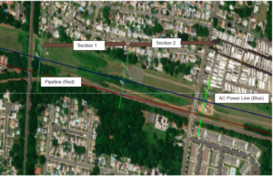
Note: The solid blue line is the pipeline and the red dashed line is the power line. Multiple power lines or pipelines can be identified by hovering over each line.

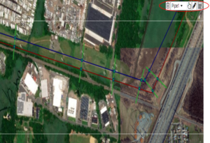
ArcGIS Map with Point and Click Automates Section Lengths, Proximities, and Angles

Once these sections are created that are based on crossings, nodes, soil resistivity, and other criteria; then calculate sections, distances, and angles steady-state and fault conditions for mitigation. To increase the resolution of the modeling, reduce section length(s). The example is a Screen Shot of Multiple Sections for Analysis. Once calculated the program will display as shown below.

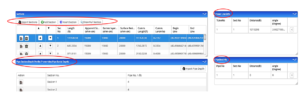
Pipeline Sectioning Data with Transmission Line Information

ArcGIS with Multiple Sections

Below is an example of sectioning created with the AC Transmission and Pipe Line Information with angles, distances, proximities, bulk soil resistivities, and depths. Once the sections are created, soil resistivities and depth of pipe data can be imported by using a template spreadsheet. In lieu of importing map data, importing soil resistivity data can also create sections using lat./long data in an Excel spreadsheet. It should be noted that section lines display the Lat/Longs.

Guideline for Determining Distance from Tower Leg to Pipeline

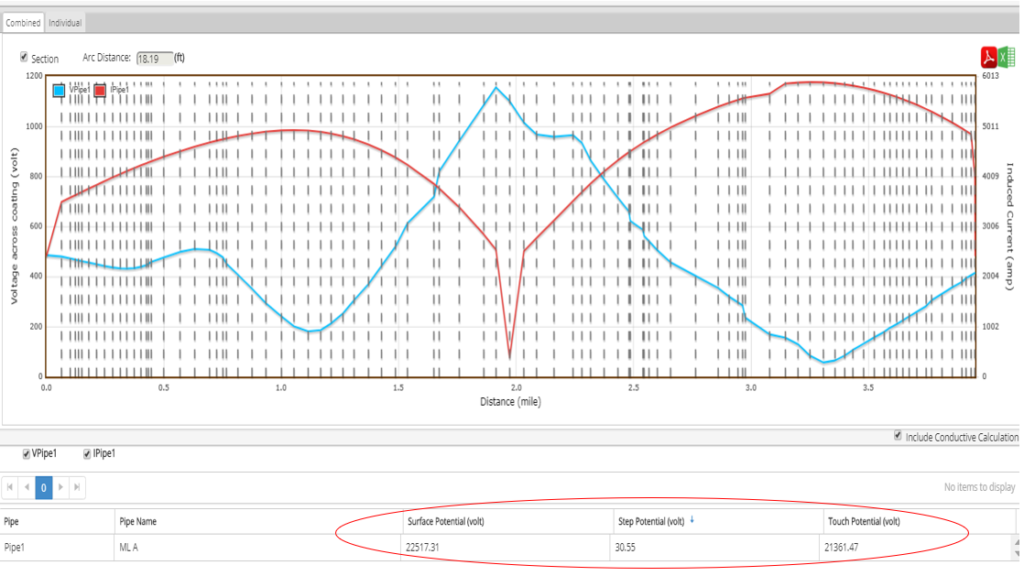
Example of a Section to Calculate Arc Distance Calculations

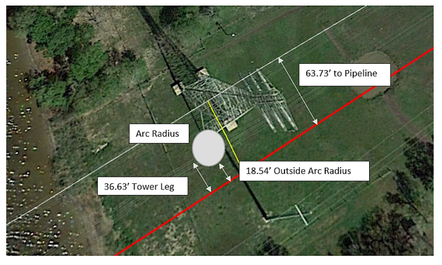
ACPT Calculations are Based on the Centerline of Tower and Pipeline (See Example Below)

• Conductive Faults dissipate directly from tower grounds to earth onto the pipe (Also call Resistive Faults and are of greater intensity)
• Inductive Faults dissipate along the shield wires and grounds to earth. (Less intensity compared to a conductive fault)
• Pipeline distance for section fault 63.73 feet from the centerline of the tower (Calculated by ACPT)
• Arc Distance calculated 18.19 feet (Blue Circle) (Calculated by ACPT) – Must be calculated from the closest leg or legs of the tower
  • Centerline distance of tower to the closest leg to pipeline (Measurement supplied by User to input UI)
    • 25’
  • To determine if a fault condition is a threat using the closest tower leg to the pipeline:
    • Calculate Distance from Centerline to Pipeline (63.73’) minus Inputted User closest leg (25’) = Actual Distance to Pipeline (36.73’)
    • Calculate Actual Leg Distance to Pipeline (36.73’) minus Arc Distance (18.19’) = Outside Influence of Arc Distance (18.54’)

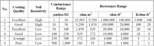
Guideline for Estimating Pipe Coating Resistance-Coating Quality

The table below is used for estimating coating resistance quality. The question that comes up is whether there are rule-of-thumb values that can be used? No, because the age and quality or condition of an FBE coating is one factor, whereas, the soil resistivity is another. When they are used together, then a more accurate assessment can be made. See table 3 below. How do assess quality:

• Excellent (Typically Less than 2 years with no change in CP current demand)
• Good (Typically greater than 2 years to 10 years and/or with small changes in CP current demand)
• Fair (Typically where the CP current demand has increased significantly from the original current requirement design)
• Poor (Typically where the CP current demand has increased significantly with major coating deterioration and high CP demand)

Table 3 – Coating Resistance Range

For more accurate coating assessments, it is recommended to run field tests for coating resistance or coating conductance. Also, see NACE Conductance test methods “Measurement of Protective Coating Electrical Conductance on Underground Pipelines”.

Note the unit conversions in table 4 below.

• (1-ohm m = 100-ohm cm)
• Coating resistance in Kohm-ft2

Table 4 – Estimating Coating Resistance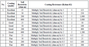
Note: Not shown above. In low resistivity soils below (2.5 ohm-m) with poor coating quality, to estimate coating resistance values use a multiplier of 0.1. Example 2.5 ohm-m x 0 .1 = 0.25 Kohm-ft2. These are estimates and it is recommended to electrically test for actual coating resistance values.

Fault Puncture Resistance

Table 5 – Coating Table

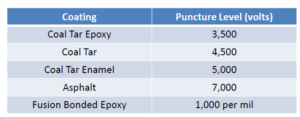To determine AC fault voltages that puncture underground pipe coatings see table 5. These are estimates and are impacted by the condition of the coating.

AC Corrosion Rates

• Greatest at holidays having a surface area of 0.155 – 0.465 in2 (1 – 3 cm2)
• High CP
• High Chloride and Alkaline environments
• DC current density rates greater than 1 am/m2

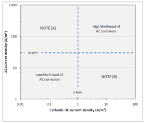
Note: There are many factors that impact the AC corrosion rate from the size of the holiday, AC and DC current density, and the environment (resistivity and make up of soils). Below is a NACE graph representing the high and low likelihoods of corrosion.

NACE Graph on AC/DC Current Density

Mitigation

The most common mitigation approach is the grounding of the pipeline by means of buried horizontal wires, galvanic anodes, etc. This is for both Steady State and Faults.

• Discrete (Ground Resistance at Node)
• Distributed (Anode Resistance Times Spacing)
• Parallel (Copper Cable(s) or zinc with De-Couplers)
• Combinations of above
• Bonding (Pipe to Pipe)

Discrete Grounds

Discrete grounding such as deep wells can be used to mitigate widely spaced voltage peaks or nodes. Nodes start at the beginning of each section typically where the pipe changes direction. If an isolating flange is located at the start/end of the line to a grounded station, a de-coupler can be used for a discrete ground to the station grounding to drain AC.

Note: Check Station Grounding for adequacy that does not interfere with SCADA and or operational instrumentation.

Distributed Vertical or Horizontal Anode Strings

These type anode strings are used at nodes or isolated voltage peaks. Example: assume a single vertical anode in a string that has a resistance to earth of 5 ohms for a 1500-foot section length with a spacing of 250 feet between anodes. The input to the program is 5 ohms x 250 spacing or 1250 as a distributed ground. By decreasing the anode separation distance and increasing the anode length/size produces a more effective grounding system. This approach can be used when multiple closely spaced voltage peaks exist on the pipeline and to isolate grounding from the CP system.

Linear (Parallel) Wire Long Line Copper Cable(s) or Zinc

Linear parallel cables are typically used as a bonded horizontal cable i.e. 1/0 or greater as the grounding element. This grounding system provides a very low impedance to ground, which results in the lowest bound to achieve satisfactory steady-state voltage levels. For example, a 2000-foot section with a horizontal 2/0 copper cable is 0.22 ohms in a 5,000 ohm-cm soil using Sunde or Dwight’s calculations. The check box in the program defaults to zinc ribbon.

• Linear (parallel) copper grounding cables with or without backfill connected to Dairyland de-couplers have a history of good performance records with trouble-free operations.
• Zinc ribbon grounding has been used in the past; however, limitations due to being part of the CP system have resulted in performance issues.
  

  Combinations of Discrete, Distributed, and Parallel

All these types of grounding can be used separately or in combination with each other. They are based on the geometry of pipes and transmission lines and soil resistivity constraints.

See Appendix B Dwight’s Curves for Grounding information for all types of the above mitigation strategies.

Pipeline Bond Connections

Pipeline bond connections are used to develop pipeline grounding capabilities for both steady-state and fault current mitigation. This approach is used when multiple closely spaced voltage peaks exist on the pipeline. However, voltage reduction is achieved with the lowest mitigation resistance in grounding. Bonding is recommended at the start and end of each section as practical.

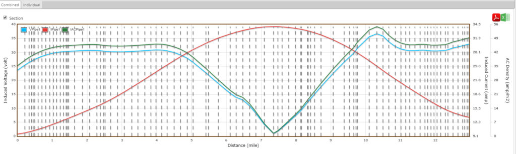
Example of Steady-State/Current Density – Unmitigated

In the graph on the next page are the results for a 30-inch diameter line, FBE coated pipeline modeled with un-mitigated Steady State volts, amps, and current density. The calculated longitudinal electrical field (LEF) under the peak current conditions is 36.71 AC volts peak AC voltage in terms of the terminating current densities of 53.99 A/m2. The field instantaneous measurement was 35 AC volts. The modeled Steady State induced AC current in the pipeline ranging from 1.5 to 54 mA. The modeled AC values were based on an isolated pipeline system on each end.

The ACPT model produced the type of results that would be expected from this type of collocated pipeline and HVPL corridor. The length of the parallel configuration, the proximity between the pipeline and HVPL, the 2300 ohm-cm soil resistivity, and the new FBE pipeline coating are all significant contributors to the modeled AC voltage and current. Steady State condition calculated and modeled a maximum of 32 volts AC at the ends of the pipeline which exceeds the 15-volt safety limit.

Where voltage safety is a concern for exposed or aboveground facilities, the use of grounding mats at test stations, above-ground valve stems, or other pipeline components. See appendix A for more details. It should be noted that these types of facilities are to be considered separately from the ACPT program. These types of mitigation are for safety and are used to discharge fault-type conditions during episodic events on the power lines. Secondary, there may be some AC currents that are discharged that may help reduce Steady State Voltages.

Example of Steady-State/Current Density-Unmitigated Graph
Example of Steady-State/Current Density – Mitigated

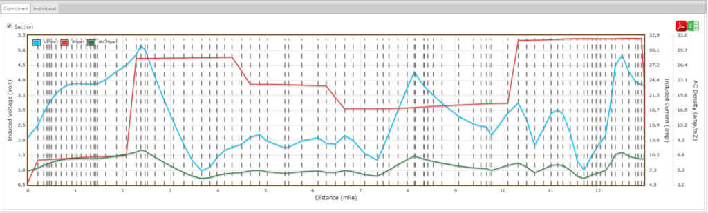
The calculated longitudinal electrical field (LEF) under the peak current loading conditions 5.3 V AC for the entire pipe segment and the mitigated peak AC voltage in terms of the terminating impedances is 4 V AC. As would be expected, the ACPT model solution had the highest calculated AC voltages at either end of the pipeline. The modeled peak AC current in the pipeline ranged from 1 to 32 Amps.

Example of Steady-State/Current Density-Mitigated Graph

The Mitigated Model using a discrete anode solution at each end and copper cable wire at peak voltages produced the type of results anticipated with the selected mitigation measures. It should be noted that steady-state voltages and current densities are now within acceptable limits to stop corrosion. See section 4.0 Corrosion Calculations for additional information.

Note: The calculated steady-state modeled voltages at both ends of the pipeline are well within the desired 15-volt safety limit.

Fault Voltage and Current – Unmitigated

Example of Graph of Fault Voltage and Current – Unmitigated

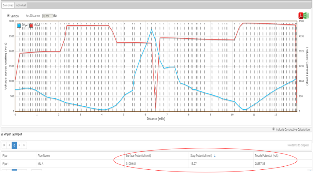Fault condition analysis was performed at several tower locations to determine the most severe condition. This severe fault condition was modeled at the end of the line where it crosses the tower lines. A maximum threshold AC voltage across the coating was modeled at 2,700 AC volts. It would require more than 14,000 volts for a 14-mil thick coating for the risk of coating damage. Based on the fault condition model results as shown below, it did require additional AC mitigation measures (discrete anode) to reduce the fault condition AC voltages for safety.

• In addition, the arc radius and surface, step, and touch potentials were calculated.
• On the next page are the results of the Peak Fault Voltages and Currents that were modeled.

Note the difference from a maximum fault on the tower to the pipeline. The graph represents the middle of the line as being the highest risk.

Fault Voltage and Current with Mitigation

ArcGIS Map with Fault Voltage and Current Mitigation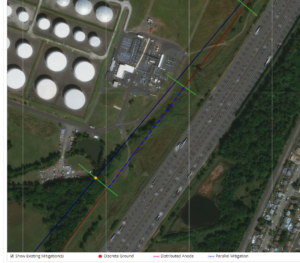

This project required a distributed anode bed on each end of the pipeline system to reduce the effects of faults where the pipeline crossed the AC tower line (See pictorial below). For personnel safety, it is recommended to use gradient control mats (GRMs) at all above-ground appurtenances such as test stations and values (See Appendix A for details). In addition, solid-state de-couplers were recommended at each of these gradient control mat sites to isolate the CP system from the grounding. The number of anodes was determined by NACE ground bed calculations for a single anode to earth and the appropriate distributed spacing.

In addition, Technical Toolboxes has a module in the Pipeline Toolbox HUB, Corrosion Control, and Cathodic Protection with a number of applications for calculating vertical and horizontal anode(s) to earth. This module also has an application for single (copper wire or zinc) linear/parallel anodes or grounds to earth.

On the next page is a linear copper grounding system (Dashed Blue Lines) with a decoupler located at a fault area (Orange Dot). By using the ArcGIS map in conjunction with planning the type of mitigation that can be installed allows the designer to make faster engineering assessments to mitigate the effects of the AC fault voltage peaks and high AC current.

AC Mitigation Design Using a Parallel Anode/Grounding System

Graph of Fault Voltage and Current – Mitigated

Below are the mitigation results for fault voltage and current. The calculated fault voltage of 1,150 VAC on the coating surface is below the effects for damage to occur based on a 5,000 VAC criterion. However, it should be noted that the surface, touch, and step potentials can present a safety risk to personnel, should a fault occur at that milli-second in time during episodic conditions. Therefore, it is always recommended to use gradient control mats for any above-ground appurtenances even with mitigation for personnel safety. Good safety practices should be implemented whenever electrical storms are in the vicinity of these facilities.

Disclaimer: Conductive Mitigated Voltage is Calculated using a PRCI Approach.

AC Corrosion Calculations

Current Density

• High AC current density effects have resulted in AC corrosion.
• AC modeling and mitigation is used to estimate AC voltage and AC current densities.
• AC current density can be calculated using a known area on a coupon (See Appendix D).
• Where:
  1. iAC = AC Current Density (A/m2)
  2. VAC = pipe AC voltage to remote earth (volt)
  3. ρ = soil resistivity (ohm-m)
  4. d = diameter of a circular holiday
• AC voltages as low as 1 VAC can produce high current densities at 1 sq. cm (0.01128) holiday in lower resistivity areas.
• AC voltage required for a current density of 100 A/m2 in 100 ohm-cm soil at a 1 sq. cm (0.01128) holiday is:

VAC = iAC x p x 3.1416 x 1sq cm (0.01128)

VAC = 0.443 Volts

Note: This calculated AC voltage is extremely low. This extreme case was shown because it happened in a brackish water crossing where a product leak occurred on a pipeline. The brackish water resistivity averaged 30 ohm/cm. This case shows the importance of understanding the risk factors and environmental conditions around the pipe.

Below is an AC chart representing these types of calculations.

AC VOLTAGE VERSUS 100 A/m2 HOLIDAY/RESISTIVITY CHART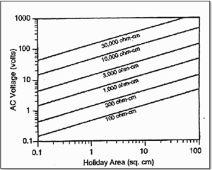

Risk of AC Corrosion Voltage Versus Resistivity

AC Voltage versus Resistivity and Multiple Iac Criteria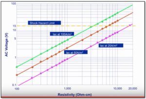

Note: See NACE documents SP0177 Latest Edition Safety Considerations and NACE 35110 State of the Art on AC Considerations for more information.

• Where AC current density is above 100 A/m2 the likelihood of AC corrosion can occur. It can also occur at lower values based on DC current density and other factors. Most engineers agree that at less than 30 A/m2 it does not occur. Below is a graph showing another version of the above graph with multiple ranges.
• In addition, the 15 VAC Shock Hazard Limit is shown.

Summary

The format developed for this AC Mitigation program makes most of the computational functions and much of the data input very easy for the designer, thus making these results understandable for unlimited pipelines and transmission towers. This is a first in this area of complex mathematical modeling. For example, data input for only one computer screen is required to exercise the program to assess the following including reporting.

• Steady-state voltage and current induction predictions
  • Current density predictions
• Fault voltage and current induction predictions
  • Step, Touch, and Surface Potentials
• Mitigation design
  • Discrete
  • Distributed
  • Parallel
• Barnes Layer (Bulk Soil Resistivity Layers)
  • Surface
  • Barnes
  • Apparent
• Depth of Cover (DOC)
• Report Generation
  • PDF
  • Spreadsheets

The AC Power Tool is an easy-to-use interface that makes the use of a HUB-based program as a viable tool for a number of potential users in your company. All pipeline functions are connected using Technical Toolboxes ArcGIS or your company’s ArcGIS.

Note: For additional AC Mitigation training, webinars, and consulting, call Technical Toolboxes or visit our website www.techncialtoolboxes.com

Example of Barnes Multi-Layer Soil Resistivity Table

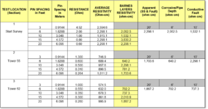Note 1: Pin Spacing can vary based on the burial depth of pipe (feet or meters) and geotechnical information. Example HDD Crossing 50′ for Corrosive Layer.

Note 2: If Pin Spacing is 5′, 10′, 15′, & 20′, use 5′ for Corrosive Layer and 10′ for Conductive (Surface Layer).

Related Links

AC Mitigation PowerTool