
The IGE Rec 3 – Low Pressure pipe flow calculator computes volumetric flow rate, pressure drop, or pipe sizing for low-pressure gas distribution systems operating at or below 1.1 psig (75 mBar). Developed by the British Gas Engineers Institute and documented in Standard IGE/TD/3, this equation is a modified version of the IGE Rec 3 – General (Medium Pressure) formulation adapted for the low-pressure regime. It uses a polynomial smooth pipe law friction factor that is Reynolds Number dependent and expresses pressure difference as a simple linear drop rather than a difference of squared pressures.
This equation is applicable only to systems operating at pressures at or below 1.1 psig (75 mBar); for higher-pressure distribution systems use the IGE Rec 3 – Medium Pressure or IGE Rec 3 – General equations.
Theory and Background
All gas pipe flow equations are ultimately derived from a general fundamental relationship: volumetric flow through a pipe segment is proportional to the pressure drop across it, divided by the combined resistance of the pipe geometry and gas properties. The greater the pressure drop, the higher the flow; the greater the resistance, the lower the flow.
The Institution of Gas Engineers and Managers (IGEM) Recommendation 3 series provides three related equations tailored to different pressure bands in British gas distribution practice. The three variants are:
| Equation | Pressure Range | ΔP Form |
|---|---|---|
| IGE Rec 3 – Low Pressure | ≤ 1.1 psig (75 mBar) | P₁ − P₂ (linear) |
| IGE Rec 3 – Medium Pressure | > 1.1 psig (75 mBar) to ≤ 29 psig (2 bar) | P₁² − P₂² (squared) |
| IGE Rec 3 – General | ≤ 101.5 psig (7 bar) | P₁² − P₂² (squared) |
At low pressures (at or below approximately 1.1 psig), the difference between gauge and absolute pressures is relatively large, meaning the squared-pressure form (P₁² − P₂²) can introduce error. The Low Pressure variant therefore uses a simple linear pressure difference (P₁ − P₂), which is a more appropriate approximation in this regime. This is the key structural distinction between the Low Pressure and Medium Pressure variants of the IGE Rec 3 equation.
Reynolds Number Dependence
Like the Medium Pressure variant, the Low Pressure equation is Reynolds Number dependent — the smooth pipe law friction factor is a function of the Reynolds Number. This means results are sensitive to gas viscosity, flow rate, and pipe diameter. The friction factor is computed via a polynomial approximation to the smooth pipe curve, making the equation explicit (non-iterative) while still capturing the Reynolds Number dependence of the partially turbulent regime.
Elevation Adjustment
When an elevation difference exists between the inlet and outlet of a pipe segment where the pressure difference is expressed as P₁² − P₂², the ΔP term is replaced with an elevation-corrected form. For the IGE Rec 3 – Low Pressure equation the pressure difference is expressed linearly (P₁ − P₂), so the standard elevation adjustment using the S-factor applies to the squared-pressure equations (Medium Pressure and General variants). Users should consult the elevation adjustment documentation within GASCalc when elevation differences are significant in low-pressure applications.
Equivalent Length Adjustment
When pipe fittings or components with different equivalent diameters are combined in a single calculation, their equivalent lengths are adjusted to a common reference diameter. For the IGE Rec 3 – Low Pressure equation, the diameter exponent used in this adjustment is 5.000 (the default for all equations other than IGT-Improved, Mueller, Panhandle-A, and Panhandle-B):
L_{EQ} = L \times \left[\frac{D_{EQ}}{D}\right]^{5.000}L_{EQ} = L \times \left[\frac{D_{EQ}}{D}\right]^{5.000}
Where:
LEQ = Adjusted equivalent length, feet
L = Original length or equivalent length associated with D, feet
DEQ = Target equivalent diameter, inches
D = Original diameter or equivalent diameter associated with L, inches
IGE Rec 3 – Low Pressure Flow Equation
As implemented in GASCalc, the Institution of Gas Engineers Recommendation 3 – Low Pressure flow equation is:
Q = 165.94 \times \frac{T_B}{P_B^{0.5}} \times \left(\frac{1}{f_{spl}}\right)^{0.5} \times \left(\frac{\Delta P}{SG \times T_F \times L \times Z}\right)^{0.5} \times D^{2.5} \times EQ = 165.94 \times \frac{T_B}{P_B^{0.5}} \times \left(\frac{1}{f_{spl}}\right)^{0.5} \times \left(\frac{\Delta P}{SG \times T_F \times L \times Z}\right)^{0.5} \times D^{2.5} \times E
Where:
Q = Volumetric flow rate at the specified base pressure and temperature, cfh
TB = Base temperature, Rankine
PB = Base pressure, psia
fspl = Smooth pipe law friction factor, dimensionless
ΔP = Pressure drop across the pipe segment (linear), psia
SG = Specific gravity, dimensionless
TF = Average gas flowing temperature, Rankine
L = Pipe length, feet
Z = Compressibility factor, dimensionless
D = Inside pipe diameter, inches
E = Pipe efficiency, decimal
Pressure Difference Term
A critical distinction of the Low Pressure variant is that ΔP is expressed as a linear pressure difference rather than a difference of squared pressures:
\Delta P = P_1 - P_2
\Delta P = P_1 – P_2
Where:
P1 = Pipe inlet (upstream) pressure, psia
P2 = Pipe outlet (downstream) pressure, psia
This contrasts with the Medium Pressure and General variants, which use ΔP = P₁² − P₂². The linear form is appropriate at low pressures where the absolute pressure values are small relative to atmospheric pressure, and the squared-pressure approximation would introduce meaningful error.
Smooth Pipe Law Friction Factor
The smooth pipe law friction factor is computed using the same polynomial approximation as the IGE Rec 3 – Medium Pressure equation. The transmission factor (1/fspl)^0.5 is expressed as an explicit polynomial function of the logarithm of the Reynolds Number, avoiding the iterative solution required by the AGA Partially Turbulent smooth pipe law:
\left(\frac{1}{f_{spl}}\right)^{0.5} = 14.7519 + 3.5657X + 0.0362X^2\left(\frac{1}{f_{spl}}\right)^{0.5} = 14.7519 + 3.5657X + 0.0362X^2
Where the Reynolds Number argument X is defined as:
X = \log_{10}(Re) - 5X = \log_{10}(Re) – 5
Where:
fspl = Smooth pipe law friction factor, dimensionless
X = Shifted log-Reynolds Number argument, dimensionless
Re = Reynolds Number, dimensionless
Because X is centered on log₁₀(Re) = 5 (i.e., Re = 100,000), the polynomial is well-conditioned for the Reynolds Numbers typical of low-pressure distribution systems. The quadratic polynomial form provides a compact, accurate approximation to the smooth pipe law curve across the applicable range without requiring iterative solution.
Comparison: IGE Rec 3 Low Pressure vs. Medium Pressure
The Low Pressure and Medium Pressure variants share the same friction factor formulation but differ in their pressure difference expression and leading coefficient, reflecting the different physical regimes. The Medium Pressure form uses:
Q = 117.3 \times \frac{T_B}{P_B} \times \left(\frac{1}{f_{spl}}\right)^{0.5} \times \left(\frac{\Delta P}{SG \times T_F \times L \times Z}\right)^{0.5} \times D^{2.5} \times E \quad (\Delta P = P_1^2 - P_2^2)Q = 117.3 \times \frac{T_B}{P_B} \times \left(\frac{1}{f_{spl}}\right)^{0.5} \times \left(\frac{\Delta P}{SG \times T_F \times L \times Z}\right)^{0.5} \times D^{2.5} \times E \quad (\Delta P = P_1^2 – P_2^2)
The Low Pressure form substitutes the linear ΔP = P₁ − P₂ and adjusts the leading coefficient and base pressure exponent accordingly (165.94 and PB0.5 vs. 117.3 and PB). This ensures dimensional consistency when switching from squared-pressure to linear-pressure units. Users should select the appropriate variant based solely on the operating pressure of the system being analyzed.
Gas Properties and Compressibility
The equation includes terms for specific gravity (SG), average flowing temperature (TF), and compressibility factor (Z). At the low pressures applicable to this equation, compressibility deviates very little from unity (Z ≈ 1.0), and in many practical low-pressure distribution calculations compressibility is set to 1.0 with negligible error. However, GASCalc supports full compressibility calculation if a compressibility factor method is specified in the Base Conditions screen.
Pipe Efficiency
All GASCalc pipe flow equations include a hydraulic efficiency term (E) to allow tuning against field measurements. For most distribution applications an efficiency of 1.0 or slightly below is appropriate. If an efficiency below 0.80 or above 1.20 is required to match field values, this typically indicates either a data entry issue or a poor equation choice for the application.
Equation Variables
Unless otherwise noted, all variables use the following base units:
D = Inside pipe diameter, inches
DEQ = Equivalent diameter associated with LEQ, inches
E = Pipe efficiency, decimal
E1 = Pipe inlet (upstream) elevation, feet
E2 = Pipe outlet (downstream) elevation, feet
fspl = Smooth pipe law friction factor, dimensionless
L = Pipe length, feet
LEQ = Equivalent length, feet
μ = Absolute viscosity, lbm/ft-sec
ΔP = Pressure drop across a pipe segment, psia (linear)
P1 = Pipe inlet (upstream) pressure, psia
P2 = Pipe outlet (downstream) pressure, psia
PATM = Average atmospheric pressure, psia
PAVE = Average pressure along the pipeline segment, psia
PB = Base pressure, psia
Q = Volumetric flow rate at the specified base pressure and temperature, cfh
Re = Reynolds Number, dimensionless
SG = Specific gravity, dimensionless
TB = Base temperature, Rankine
TF = Average gas flowing temperature, Rankine
X = Shifted log-Reynolds Number argument = log₁₀(Re) − 5, dimensionless
Z = Compressibility factor, dimensionless
Case Guide
Part 1: Create Case
- Select the IGE Rec 3 – Low Pressure application from the Hydraulics Module.
- To create a new case, click the “Add Case” button.
- Enter a Case Name, Location, Date, and any necessary notes.
- Click the Base Conditions command button. Set the appropriate base pressure, base temperature, gas properties file, atmospheric pressure method, and compressibility factor method. For most low-pressure applications, the Compressibility Factor Method may be set to “None” (Z = 1.0).
- From the Pipe Flow Equation list, confirm IGE Rec 3 – Low Pressure is selected.
- Click on the red label of the item to be calculated (the “unknown” value) until the label is underlined. Only one unknown may be selected at a time.
- Select the appropriate dimensional units for all data items.
- Enter values for all known parameters: Diameter, Length, Efficiency, Flow Rate, Inlet Pressure, Outlet Pressure, Inlet Elevation, Outlet Elevation, Inlet Temperature, and Outlet Temperature as applicable.
- If fittings are to be included, add them using the Additional Components panel on the Other Data tab.
- Click the CALCULATE button to compute results.
Input Parameters
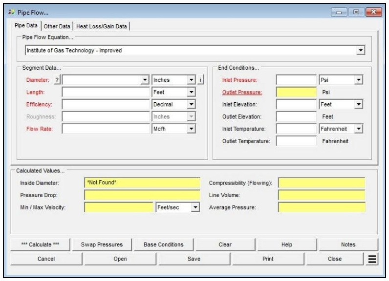
| Parameter | Description |
|---|---|
| Pipe Flow Equation | Specifies the flow equation to use. Select IGE Rec 3 – Low Pressure from the drop-down list. |
| Diameter | Specifies or displays the hydraulic (inside) diameter of the pipe segment. Click the ? button to select a size using the Pipe Selection screen. May be designated the unknown to solve for. |
| Length | Specifies or displays the hydraulic length of the pipe segment. May be designated the unknown to solve for. |
| Efficiency | Specifies or displays the hydraulic efficiency of the pipe segment (decimal). Typical values are 0.80–1.20; values outside this range may indicate a data or equation mismatch. |
| Roughness | Specifies the internal wall roughness of the pipe segment (inches). Not used by the IGE Rec 3 – Low Pressure equation; field is disabled for this equation selection. |
| Flow Rate | Specifies or displays the volumetric flow rate through the pipe segment, expressed in standard volume units at base conditions. May be designated the unknown to solve for. |
| Inlet Pressure | Specifies or displays the gauge pressure at the inlet (upstream) end of the pipe segment. May be designated the unknown to solve for. |
| Outlet Pressure | Specifies or displays the gauge pressure at the outlet (downstream) end of the pipe segment. May be designated the unknown to solve for. |
| Inlet Elevation | Specifies the height above mean sea level at the inlet end of the pipe segment. Displayed and enabled when the Atmospheric Pressure Method is not set to “None” or “None – Entered Value.” |
| Outlet Elevation | Specifies the height above mean sea level at the outlet end of the pipe segment. Displayed and enabled when the Atmospheric Pressure Method is not set to “None” or “None – Entered Value.” |
| Inlet Temperature | Specifies the flowing gas temperature at the inlet (upstream) end of the pipe segment. |
| Outlet Temperature | Specifies the flowing gas temperature at the outlet (downstream) end. Only calculated when the Heat Loss/Gain method is active or Joule-Thomson cooling is selected. |
Part 2: Outputs/Reports
- If you need to modify an input parameter, click the CALCULATE button after the change.
- To SAVE, fill out all required case details then click the SAVE button.
- To rename an existing file, click the SAVE As button. Provide all case info then click SAVE.
- To generate a REPORT, click the REPORT button.
- The user may export the Case/Report by clicking the Export to Excel icon.
- To delete a case, click the DELETE icon near the top of the widget.
Results
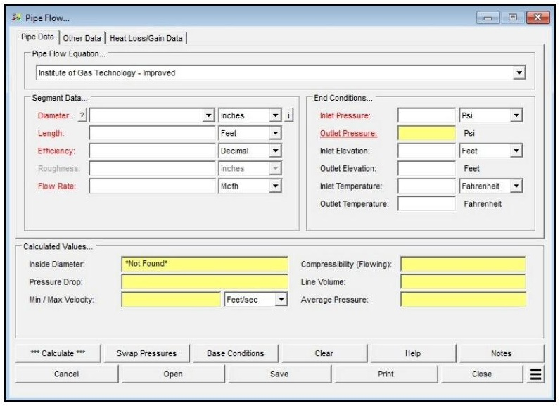
| Output | Description |
|---|---|
| Solved Unknown | Displays the calculated value of whichever parameter was designated the unknown — Diameter, Length, Flow Rate, Inlet Pressure, or Outlet Pressure — in the units specified for that item. |
| Inside Diameter | Displays the inside diameter of the pipe segment when a Size/Type Code is used to specify the Diameter value. Read from the Pipe Property Table. |
| Pressure Drop | Displays the calculated linear pressure drop across the pipe segment, including all attached components (psi or millibar). For the Low Pressure variant this is expressed as P₁ − P₂. |
| Min / Max Velocity | Displays the calculated minimum and maximum flow velocity in the pipe segment. The minimum is calculated at inlet conditions; the maximum at outlet conditions (ft/sec or m/sec). |
| Compressibility (Flowing) | Displays the calculated average flowing compressibility factor, computed from the average pressure and temperature along the segment. Typically very close to 1.0 at low-pressure operating conditions. |
| Line Volume | Displays the calculated volume of gas contained in the pipe segment at base conditions. Computed from average pressure, temperature, and compressibility factor values (Mcf or m³). |
| Average Pressure | Displays the calculated average pressure along the pipe segment (psia or millibar). Used internally to compute Compressibility (Flowing) and Line Volume. |

References
- The Institution of Gas Engineers and Managers, Steel and PE Pipelines For Gas Distribution, Recommendations on Transmission and Distribution Practice, Standard IGE/TD/3 Edition 4, 2003.
- Gas Processors Suppliers Association, Engineering Data Book, Eleventh Edition – FPS, 1998.
- Industrial Press, Gas Engineers Handbook, 1965.
- GASCalc 6.1 Calculation Reference – Pipe Flow, Revision 005, Copyright 2025.
FAQ
-
Gas Purging Calculations?
Purging is a process of removing gas from the pipeline. Controlled purging of gases from pipelines by direct displacement with other gases that have been safely practiced for many years with the recognition that some flammable mixture is present. Purging of gases from pipelines by direct displacement with another gas also has been similarly practiced. It works both ways; however, there will always be an atmosphere of type of a mixture. This is due to the densities of the gases. Check Out
-
What is Erosional Velocity?
Pipe erosion begins when velocity exceeds the value of C/SQRT(ρ) in ft/s, where ρ = gas density (in lb./ft3) and C = empirical constant (in lb./s/ft2) (starting erosional velocity). We used C=100 as API RP 14E (1984). However, this value can be changed based on the internal conditions of the pipeline. Check Out
-
What is Sonic Velocity?
The maximum possible velocity of a compressible fluid in a pipe is called sonic velocity. Oilfield liquids are semi-compressible, due to dissolved gases. Check Out
-
What is Pipe Roughness?
Pipe roughness is a material property that refers to the absolute roughness of the internal pipe wall surface, used in friction factor calculations for pressure drop and flow calculations. These roughness values may be auto-populated by selecting the “Select Pipe Roughness” dropdown, or by manually inputting the value specified by the manufacturer.